Barium II – ChETEC-INFRA

Description of how barium abundance corrections have been obtained and how to use them as a PDF document can be found here or below. You can download entire database in ASCII here.

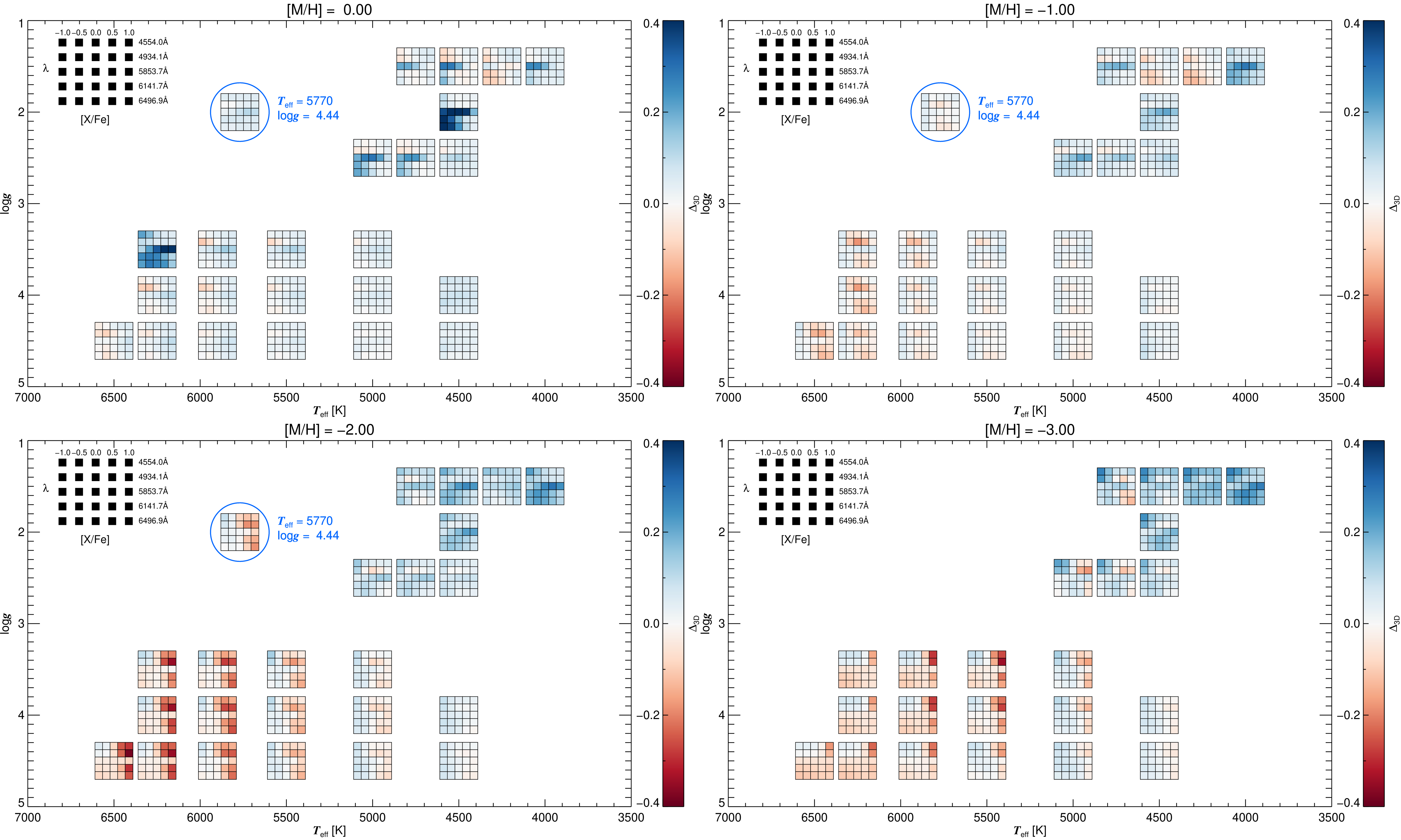
Figure 1. 3D NLTE – 1D LTE abundance corrections for different Ba II spectral lines. If applied to [Ba/Fe] obtained by the LTE spectrum synthesis using a MARCS model atmosphere, would obtain abundance estimate as if using NLTE spectrum synthesis with a virtual 3D MARCS model atmosphere. One must interpolate the corrections using the 3D NLTE equivalent widths to extract the 3D virtual MARCS correction needed for a given 1D abundance. Click on a square to open a correction table for those atmospheric parameters in a new window.

When dealing with a particular line at a given T_eff / log g / [M/H] and A(Ba), one only requires up to 4 tables if the log g and [M/H] is between them. By interpolating over temperature first for a given line, then by gravity and finally by [Ba/Fe], then user can interpolate to the correct metallicity. Tables for particular log g and [M/H] combinations can be found in the table bellow (containing multiple T_eff and A(Ba) values).

log g	[M/H] = 0.0	[M/H] = -1.0	[M/H] = -2.0	[M/H] = -3.0
1.5	download	download	download	download
2.0	download	download	download	download
2.5	download	download	download	download
3.5	download	download	download	download
4.0	download	download	download	download
4.4	download	download	download
4.5	download	download	download	download

1. Overview

We present a grid of 3D NLTE – 1D LTE abundance corrections for a number of barium spectral lines for a sequence of F, G, and K dwarf and giant stellar model atmospheres. Following standard convention here, (N)LTE stands for (non-)Local Thermodynamic Equilibrium. The corrections can be used to improve the accuracy of the barium abundance obtained by standard 1D LTE techniques by applying the tabulated corrections, thus accounting for the combined effect of the 3D atmospheric structure and deviations of the atomic level populations from local thermodynamic equilibrium. We also present a corresponding grid of 1D NLTE — 1D LTE abundance corrections.

To reduce the computational costs, we have adopted the so-called 1.5D approximation for computing the level populations only, i.e., we treat each column of the 3D models atmosphere as an independent plane-parallel 1D model when solving the statistical equilibrium. Using the 1.5D departure coefficients, the final line formation is computed on the full 3D structure, including the hydrodynamical velocity field. In this sense, we refer to 3D NLTE results in the following. Our assumption that the 1.5D departure coefficients are a very good approximation of the full 3D departure coefficients is based on previous results for other chemical elements. The validity of the 1.5D approximation for the case of barium is presently being investigated in a separate study.

The tabulated corrections were created using two codes: the 1.5D statistical equilibrium code NLTE15D, and the 3D spectral synthesis code Linfor3D. NLTE15D is an MPI wrapper that allows one to solve the 1D statistical equilibrium problem on every vertical column of a 3D model. It uses the 1D statistical equilibrium code Multi 2.3 (Carlsson, 1986). NLTE15D works for both 3D and 1D model atmospheres. The 1.5D departure coefficient data computed with NTLE15D is used as input into Linfor3D to perform a full 3D NLTE spectrum synthesis. Matching the resulting line strengths with 1D LTE line profiles obtained from the associated 1D reference model atmosphere sharing the same stellar parameters yields the desired 3D NLTE — 1D LTE abundance corrections.

A small description of each code can be found in Appendices A & B. A detailed breakdown of Linfor3D can be found in the Linfor3D user manual.

Special care has been taken regarding the choice of the 1D reference model atmospheres and a consistent treatment of the microturbulence. In the following, we shall briefly discuss these important aspects for preparing and using our abundance correction grids.

References:
Carlsson, M. 1986, Uppsala Astronomical Observatory Reports, 33

2. Corrections computations

This section describes the adopted method for computing 3D abundance corrections. In principle, the method presented below can be applied to any 3D model atmosphere, e.g. CO⁵BOLD, Stagger, etc., and any 1D model atmosphere, e.g. MARCS, ATLAS, PHOENIX, MAFAGS, etc. In this study we will describe this method in the context of CO⁵BOLD and MARCS models.

To compute 3D abundance corrections, one usually relies on an associated 1D reference model that has the same stellar parameters (T_eff, log g, and [M/H]) and uses the same equation-of-state (EOS), opacities and radiative transfer scheme as the related 3D model. In contrast to the 3D model, convection is treated by the mixing-length formalism in the 1D model. When using the 1D model for computing 1D LTE (or NLTE) line profiles, non-thermal line broadening is described by a depth-independent microturbulence velocity, ξ_micro (see Sect. Microturbulence). In the context of CO⁵BOLD, the associated 1D models are so-called LHD models. The idea is that the abundance corrections derived from a strictly differential comparison of CO⁵BOLD 3D NLTE and LHD 1D LTE spectra would be largely independent of the detailed microphysics, provided that it is identical in the 3D and the 1D models. In practice, this would mean that the corrections based on CO⁵BOLD–LHD models could be applied directly to 1D LTE abundances derived from any 1D model to obtain 3D NLTE abundances that would be produced by the related virtual 3D model atmosphere with the same microphysics.

Unfortunately, it turns out that the assumption that the 3D NLTE–1D LTE abundance corrections are insensitive to the EOS and opacities employed in the construction of both the 3D and the associated 1D model is not strictly valid. This is obvious from the fact that the 1D NLTE–1D LTE corrections are systematically different between LHD and MARCS models (see Harutyunyan et al., 2018, their Sect. 2.6, and Mott et al., 2020, their Fig. 15). This means that applying the 1D NLTE corrections based on LHD models to the 1D LTE abundances derived with 1D MARCS models does not give the correct MARCS 1D NLTE abundance. Likewise, applying the 3D NLTE corrections based on CO⁵BOLD–LHD models to the 1D LTE abundances derived with 1D MARCS models would not give the correct 3D NLTE abundance of a virtual 3D MARCS model atmosphere.

References:
Harutyunyan, G., Steffen, M., Mott, A., et al. 2018, A&A, 618, A16.
Mott, A., Steffen, M., Caffau, E., et al. 2020, A&A, 638, A58.

2.1. Corrected corrections

This problem may be addressed by correcting the corrections as follows. Define the abundance corrections obtained from 3D/1D models with microphysics 0 and 1, respectively as

(1) $\begin{equation*}\Delta^0_{\rm 3D} &= A{\rm (X)}^0_{\rm 3D\,NLTE} - A{\rm (X)}^0_{\rm 1D\,LTE}\ &= A{\rm (X)}^0_{\rm 3D\,NLTE} - A{\rm (X)}^0_{\rm 1D\,NLTE} + \left( A{\rm(X)}^0_{\rm 1D\,NLTE} - A{\rm (X)}^0_{\rm 1D\,LTE} \right)\, ,\end{equation*}$

(2) $\begin{equation*}\Delta^1_{\rm 3D} &= A{\rm (X)}^1_{\rm 3D\,NLTE} - A{\rm (X)}^1_{\rm 1D\,LTE}\ &= A{\rm (X)}^1_{\rm 3D\,NLTE} - A{\rm (X)}^1_{\rm 1D\,NLTE} + \left( A{\rm(X)}^1_{\rm 1D\,NLTE} - A{\rm (X)}^1_{\rm 1D\,LTE} \right)\, ,\end{equation*}$

where $A{\rm (X)}$ is the logarithmic abundance of element X, defined as

$\begin{equation*} A{\rm (X)} = \log_{10}{\frac{N{\rm (X)}}{N{\rm (H)}}} + 12\, . \end{equation*}$

The different abundances are defined by requiring the equality of line equivalent widths $EW$

$\begin{equation*} EW_{\rm 3D\,NLTE}(A{\rm (X)}_{\rm 3D\,NLTE}) = EW_{\rm 1D\,NLTE}(A{\rm (X)}_{\rm 1D\,NLTE}) = EW_{\rm 1D\,LTE}(A{\rm (X)}_{\rm 1D\,LTE})\, .\end{equation*}$

In this document, Eq.~(1) refers to \cobold\ models and Eq.~(2) to MARCS EOS and opacities. The question is then how to obtain the unknown 3D NLTE MARCS abundance correction, $\Delta_{\rm 3D}^1$ , from the known standard \cobold–LHD 3D NLTE correction, $\Delta_{\rm 3D}^0$ .

If instead of assuming $\Delta_{\rm 3D}^1 \approx \Delta_{\rm 3D}^0$ , which turned out not to be strictly valid, we instead make the assumption

(3) $\begin{equation*}A{\rm (X)}^1_{\rm 3D\,NLTE} - A{\rm (X)}^1_{\rm 1D\,NLTE} \approx A{\rm(X)}^0_{\rm 3D\,NLTE} - A{\rm (X)}^0_{\rm 1D\,NLTE}\, ,\end{equation*}$

which is presumably a much better approximation of the real interplay between these models, it leads us to

(4) $\begin{equation*}\Delta^1_{\rm 3D} &= A{\rm (X)}^1_{\rm 3D\,NLTE} - A{\rm (X)}^1_{\rm 1D\,LTE}\ &= \Delta^0_{\rm 3D} - \left( A{\rm (X)}^0_{\rm 1D\,NLTE} - A{\rm(X)}^0_{\rm 1D\,LTE} \right) + \left( A{\rm (X)}^1_{\rm 1D\,NLTE} - A{\rm(X)}^1_{\rm 1D\,LTE} \right)\, ,\end{equation*}$

or, in short,

(5) $\begin{equation*}\Delta^1_{\rm 3D} = \Delta^0_{\rm 3D} + \left( \Delta^1_{\rm 1D} -\Delta^0_{\rm 1D} \right)\, .\end{equation*}$

Therefore, when performing a 1D LTE analysis with MARCS models, the standard 3D NLTE corrections, $\Delta^0_{\rm 3D}$ , must be corrected by the difference of the 1D NLTE corrections $\left( \Delta^1_{\rm 1D} - \Delta^0_{\rm 1D} \right)$ , henceforth known as the correction factor. We note that this correction term has the wrong sign in Matas Pinto et al. (2021), but their final result is fortunately correct, nevertheless.

As a consequence of this consideration, we have computed 3D NLTE corrections using CO⁵BOLD and LHD model atmospheres, $\Delta^0_{\rm 3D}$ , 1D NLTE corrections using LHD model atmospheres, $\Delta^0_{\rm 1D}$ , and 1D NLTE corrections using MARCS model atmospheres, $\Delta^1_{\rm 1D}$ . The 3D corrections presented in the associated tables (column 3D_corr) provide the virtual 3D MARCS corrections, $\Delta^1_{\rm 3D}$ . By design, application of this correction factor to the standard 1D LTE abundance derived from a MARCS model atmosphere for a particular spectral line yields the final corrected abundance that is equivalent to what would have been obtained from a full 3D NLTE analysis.

For completeness, the correction factor is given in column c_factor, which means that it is possible to recover $\Delta^0_{\rm 3D}$ . Further details concerning the contents of the correction tables can be found in Sect. 7.

References:
Matas Pinto, A. M., Spite, M., Caffau, E., et al. 2021, A&A, 654, A170.

3. 3D model atmospheres

The 3D models used for this project are from a precomputed grid of 3D models that were computed with the 3D radiation hydrodynamics code CO⁵BOLD (Freytag et al., 2012). Many of them come from the CIFIST model grid (Ludwig et al., 2009). So that these correction grids can be used for a variety of studies, we have made sure to cover a reasonable range in effective temperature, T_eff, gravity, log g, and metallicity, [M/H]. At present, the correction grid includes dwarfs and giants of spectral type F, G, and K over a temperature range of

$\begin{equation*}4000 \leq T_{\rm eff} \ {\rm [K]} \leq 6500\end{equation*}$

for a range in gravity of

$\begin{equation*}1.5 \leq \log{g} \leq 4.5\end{equation*}$

for four metallicities over the range

$\begin{equation*}-3.0\leq{\rm [M/H]}\leq+0.0, \qquad\qquad {\rm where} \; \Delta {\rm [M/H]} = 1.0\,{\rm dex}\end{equation*}$

with

$\begin{equation*}{\rm [X/Y]} &= {\rm [X/H]} - {\rm [Y/H]} \ &= \left( A{\rm (X)}{} - A{\rm(X)}_\odot \right) - \left( A{\rm (Y)}{} - A{\rm (Y)}_\odot \right)\, .\end{equation*}$

Each 3D model consists of a series of representative snapshots in time. The number of snapshots for each hydrodynamical simulation is 20, with some exceptions having 8, 12, 18, 19, or 21 snapshots instead. Every snapshot was included in the statistical equilibrium and spectrum synthesis computations with NLTE15D and Linfor3D, respectively. In addition, the corresponding 1D LHD model was also used as input to Linfor3D (in LTE mode) for computing 3D NLTE abundance corrections, $\Delta_{\rm 3D}^0$ , according to Eq. (1, Sect. 2.1).

References:
Freytag, B., Steffen, M., Ludwig, H.-G., et al. 2012, Journal of Computational Physics, 231, 919.
Ludwig, H.-G., Caffau, E., Steffen, M., et al. 2009, Mem. Soc. Astron. Ital., 80, 711.

4. 1D model atmospheres

To compute the corrected corrections according to Eq. (5, Sect. 2.1), we performed statistical equilibrium computations with 1D LHD and 1D MARCS models (Gustafsson et al., 2008). Every 3D model selected for this study came with a dedicated LHD model specially computed for the 3D model’s stellar parameters (T_eff, log g, and [M/H]) with the same microphysics used by the 3D model. To get a 1D MARCS model with identical stellar parameters, an interpolation routine written by Thomas Masseron was used. This is downloadable at https://marcs.astro.uu.se/software.php. Every 1D LHD and interpolated 1D MARCS model was then used as input for NLTE15D to compute 1D level population departure coefficients. Those departures were subsequently used with the respective 1D models as input to Linfor3D where the required 1D NLTE abundance corrections were computed ( $\Delta_{\rm 1D}^0$ and $\Delta_{\rm 1D}^1$ in Eq. 5, Sect. 2.1).

References:
Gustafsson, B., Edvardsson, B., Eriksson, K., et al. 2008, A&A, 486, 951.

5. Microturbulence

As abundance corrections require the use of 1D models, and because we solve the statistical equilibrium equations using the 1.5D rather than 3D method, microturbulence remains an important quantity, unless the spectral lines under investigations are weak.

For the present purpose, we decided to define a depth-independent microturbulence, $\xi_{\rm micro}^{\rm 3D}$ (T_eff, log g, and [M/H]) which is a function of the stellar parameters but is identical for all columns of the 1.5D statistical equilibrium computations and is also employed in the 1D reference models used for the abundance correction computations. The idea is to choose $\xi_{\rm micro}^{\rm 3D}$ such that it represents the effective microturbulence defined by the hydrodynamical velocity field of the respective 3D model atmosphere. This implies that microturbulence is not another independent parameter of the abundance correction grid, as it is uniquely linked to the stellar parameters.

For computing $\xi_{\rm micro}^{\rm 3D}$ from the 3D velocity fields of the CO⁵BOLD models, we follow the approach suggested in Steffen et al. (2013), their Appendix A. In this context we adopt a set of weighting functions representing the different line formation regions of typical iron lines. We take the variation of the resulting $\xi_{\rm micro}^{\rm 3D}$ over the set of weighting function as a measure of the associated microturbulence uncertainty. This allows us to compute systematic uncertainties on our abundance corrections, borne from the uncertainty to the microturbulence.

In observational studies, it is customary to determine the microturbulence from the curve-of-growth: the microturbulence is adjusted until any systematic trend with line strength of the abundance derived from different lines of the same element (usually iron) is eliminated. For an individual target, the microturbulence derived in this way, $\xi_{\rm micro}^\ast$ , will in general be different from the theoretical value computed from the 3D CO⁵BOLD model, $\xi_{\rm micro}^{\rm 3D}$ , even if the stellar parameters are identical. This is, however, not a problem: the recipe is to use $\xi_{\rm micro}^\ast$ for deriving the original 1D LTE abundance, and to subsequently improve this 1D LTE abundance by applying the tabulated 3D NLTE correction, even if the latter was computed with a different microturbulence, $\xi_{\rm micro}^{\rm 3D}$ . This procedure can be justified even if $\xi_{\rm micro}^\ast$ and $\xi_{\rm micro}^{\rm 3D}$ are significantly different. This is because, on the theoretical side, the differential approach taken in defining the 3D NLTE abundance corrections ensures that 3D and 1D reference model share the same effective microturbulence ( $\xi_{\rm micro}^{\rm 3D}$ ) while, on the observational side, the target and the 1D model used for the abundance analysis share the same microturbulence ( $\xi_{\rm micro}^\ast$ ), too.

References:
Steffen, M., Caffau, E., & Ludwig, H.-G. 2013, Memorie della Societa Astronomica Italiana Supplementi, 24, 37.

6. Barium lines

We have computed corrections for five barium abundances for every model. The absolute barium abundance varies according to the model metallicity such that

$\begin{equation*}-1.0\leq{\rm [Ba/Fe]}\leq+1.0, \qquad\qquad {\rm where} \; \Delta {\rm [Ba/Fe]} = 0.5\,{\rm dex}\, ,\end{equation*}$

and the adopted solar barium abundance is

$\begin{equation*}A{\rm (Ba)}_\odot = 2.27\end{equation*}$

as determined in Gallagher et al. (2020).

The barium model atom used for the statistical equilibrium calculations with NLTE15D was also taken from Gallagher et al. (2020), and is well described there. The resulting level population departure coefficients for five energy levels were saved from each NLTE15D run for each abundance so that they could be used as input with Linfor3D to compute 1D and 3D NLTE barium line profiles. This allowed us to compute abundance corrections for five barium lines in the optical part of the spectrum that are widely used for abundance work. Details are listed in Table 1.

Table 1: The five bound-bound transitions and their level configurations for which abundance corrections are presented in this study.

λ [Å]	lower level	upper level
4554.033	6s² S_1/2	6p²P^◦_3/2
4934.077	6s² S_1/2	6p²P^◦₁_/2
5853.688	5d²D_3/2	6p²P^◦_3/2
6141.727	5d²D_3/2	6p²P^◦_3/2
6496.910	5d²D_3/2	6p²P^◦₁_/2

All the barium lines listed in Table 1 consist of five barium isotopes, ^134-138Ba. The non-zero net nuclear spin of the odd isotopes causes hyperfine splitting (hfs) in the levels. These properties were properly included in the spectrum synthesis of every barium line. The isotopic ratio used for all barium line profiles throughout the grid was taken as solar

$\begin{equation*}{}^{134}{\rm Ba}:{}^{135}{\rm Ba}:{}^{136}{\rm Ba}:{}^{137}{\rm Ba}:{}^{138}{\rm Ba} = \left( 2.43:6.60:7.88:11.24:71.85\right) \% \, ,\end{equation*}$

according to Arlandini et al. (1999). Further details on the hfs and line lists for four of the five lines used in the present study can also be found in Gallagher et al. (2020, their Appendix A). Full details will be given in the forthcoming paper.

References:
Arlandini, C., Käppeler, F., Wisshak, K., et al. 1999, ApJ, 525, 886.
Gallagher, A. J., Bergemann, M., Collet, R., et al. 2020, A&A, 634, A55.

7. The correction tables

The various tables available consist of several columns, which are now briefly described

7.1 Teff

The model effective temperature [K].

7.2 ximic

The microturbulence $\xi_{\rm micro}^{\rm 3D}$ in [km/s] (see Sect. 5).

7.3 d_ximic

The associated uncertainty in microturbulence, $\sigma_{\xi_{\rm micro}^{\rm 3D}}$ , in [km/s] (see Sect. 5).

7.4 Wavelength

The central wavelength of the bound-bound transition in [Å].

7.5 [X/Fe]

The differential barium abundance relative to iron (X represents barium).

7.6 A(X)

The logarithmic barium abundance relative to hydrogen.

7.7 3D_corr

The 3D corrected barium abundance correction $\Delta^1_{\rm 3D}$ (see Sect. 2).

7.8 3D_sig_rand

The random error as determined by the scatter in the 3D correction due to the variability between snapshots of a given model.

7.9 3D_sig_sys_lo

The systematic error of $\Delta^1_{\rm 3D}$ due to a decrease of $\xi_{\rm micro}^{\rm 3D}$ by the uncertainty in the assigned microturbulence (columns ximic - d_ximic) computed from the 3D models (see Sect. 5).

7.10 3D_sig_sys_hi

The systematic error of $\Delta^1_{\rm 3D}$ due to an increase of $\xi_{\rm micro}$ by the uncertainty in the assigned microturbulence (columns ximic - d_ximic) computed from the 3D models (see Sect. 5).

7.11 1D_corr

The 1D NLTE MARCS abundance correction $\Delta^1_{\rm 1D}$ .

7.12 c_factor

The correction factor, ( $\Delta^1_{\rm 1D}-\Delta^0_{\rm 1D}$ ), see Eq. (5, Sect. 2.1).

7.13 EW_3DNLTE

The equivalent width of the 3D CO⁵BOLD NLTE line profile, computed with the
barium abundance given in column A(X).

7.14 EW_1DNLTE

The equivalent width of the 1D MARCS NLTE line profile, again computed with the barium abundance given in column A(X).

7.15 EW_1DLTE

The equivalent width of the 1D MARCS LTE line profile, again computed with the barium abundance given in column A(X).

8. Using the correction tables

The tables are separated according to the models’ gravity and metallicity. Each table contains the computed quantities for all five spectral lines and for every available stellar effective temperature. To use these tables correctly, one must interpolate them to the desired stellar parameter set and barium abundance.

8.1 Correcting 1D LTE data with the tables

It is important to understand that, contrary to common practice, our corrections are presently not tabulated as a function of the 1D LTE abundance $A{\rm (X)}^1_{\rm 1D\,LTE}$ but rather as a function of the 3D NLTE abundance $A{\rm (X)}^0_{\rm 3D\,NLTE}$ . For given stellar parameters (\teff, \logg, [M/H]), the path to the final corrected abundance therefore requires a deviation via equivalent width (EW) as follows

$\begin{equation*}A{\rm (X)}^1_{\rm 1D\,LTE} \rightarrow EW^1_{\rm 1D\,LTE}\equiv EW^0_{\rm 3D\,NLTE} \rightarrow \Delta^1_{\rm 3D} \rightarrow A{\rm (X)}^1_{\rm 3D\,NLTE}\,.\end{equation*}$

The first step is to evaluate the 1D LTE equivalent width corresponding to the (MARCS) 1D LTE abundance, which is then identified with the 3D NLTE equivalent width tabulated in column EW_3DNLTE. Therefore, one must interpolate the 3D abundance correction tabulated in column 3D_corr to the correct (MARCS) 1D LTE equivalent width using column EW_3DNLTE. This is depicted in Fig. 1. Finally, the interpolated correction is added to the initial 1D LTE abundance,

$\begin{equation*}A{\rm (X)}^1_{\rm 3D\,NLTE}= A{\rm (X)}^1_{\rm 1D\,LTE} + \Delta^1_{\rm 3D}\,.\end{equation*}$

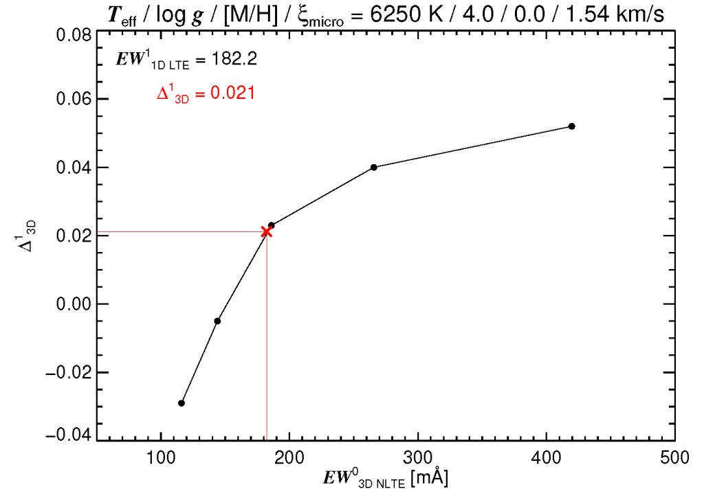
Figure 2. Example of extracting the relevant 3D NLTE correction, $\Delta^{1}_{\rm 3D}$ , for the $4554.0332$ Å line. First, the 1D LTE abundance $A{\rm (X)}^1_{\rm 3D\,NLTE}$ is adjusted such that the 1D LTE equivalent width, ${EW}^{1}_{\rm 1D LTE}$ matches the observed equivalent width, ${EW}^\ast$ . The same line strength must be reproduced in 3D NLTE, ${EW}^{0}_{\rm 3D NLTE}={EW}^\ast={EW}^{1}_{\rm 1D LTE}$ . The relevant 3D correction is then found by interpolation of the plotted relation, column (7) versus column (13) to determine $\Delta^{1}_{\rm 3D}$ at ${EW}^{0}_{\rm 3D NLTE}={EW}^{1}_{\rm 1D LTE}$ .

8.2 Uncertainties

Each 3D correction has an associated random and systematic uncertainty

$\begin{equation*}\Delta^{+c}_{-b}\pm a\, ,\end{equation*}$

where $a$ is the random uncertainty listed in column 3D_sig_rand, $b$ is the lower systematic uncertainty listed in column 3D_sig_sys_lo, and $c$ is the upper systematic uncertainty listed in column 3D_sig_sys_hi. The uncertainties can be added in quadrature to the existing abundance uncertainty from the 1D LTE analysis to provide a 3D NLTE abundance with an associated uncertainty. They can also be used to assess the confidence one can assign the given correction. While the error associated with the snapshot variability will remain consistently low, the systematic uncertainty from the microturbulence will vary according to the sensitivity of that line computed in 1D at a given barium abundance for a given 1D model to the microturbulence. If the line is very weak or very strong this sensitivity is severely diminished and the uncertainty will be small. However, lines of intermediate strength approaching saturation can be heavily influenced by the uncertainty in the microturbulence and will have a large systematic uncertainty to the correction.

8.3 Citing the correction tables

The correction tables are available to all to use freely. A paper further describing the computations and correction grid is forthcoming. For the moment, we ask that you cite this webpage and include the following text in the acknowledgements:

“The (1D NLTE/3D NLTE) corrections used in this work were provided by the ChETEC-INFRA project (EU project no. 101008324), task 5.1.”

Please delete or adjust “(1D NLTE/3D NLTE)” as appropriate.

Appendix A. NLTE15D

NLTE15D is a MPI wrapper designed to work with existing 1D statistical equilibrium codes such as Multi (Carlsson, 1986). It is able to read 3D hydrodynamical models from both CO⁵BOLD and STAGGER. A 3D model is read and each vertical column is treated as an individual 1D model when it is parsed to a Multi session, which computes the 1D statistical equilibrium for that “1D model”. This method is known as 1.5D statistical equilibrium.

Once the Multi session has completed, the output data is returned to NLTE15D, which then creates the level population departure coefficients and stores them in the corresponding vertical column in a 3D data cube. Once each column has been computed, NLTE15D saves the data in a format that is readable by the 3D spectral synthesis code, Linfor3D.

The code can split horizontal grid into parallel jobs according to the number of CPUs set. Each CPU is given a subset of vertical columns according to how the code has split the horizontal grid. This has proved to be very scalable on large computing facilities as there is very little communication between CPUs.

The code is very new, but has been through substantial phases in testing before it was used in this project. However, a user manual is not yet available, but is being prepared.

References:
Carlsson, M. 1986, Uppsala Astronomical Observatory Reports, 33

Appendix B. Linfor3D

Linfor3D is a 3D spectral synthesis code, which is capable of computing spectral lines or spectral regions in both LTE and NLTE. The latter is possible if departure coefficient data exists for a given bound-bound transition. For the context of this work, Linfor3D was used to compute 1D and 3D NLTE abundance corrections for five barium transitions. Linfor3D performs this computation internally by creating a 1D LTE curve-of-growth (CoG) over abundance range set by the user, centered on the input abundance. The 1D abundance required to reproduce the 3D (NLTE) equivalent width is determined via interpolation across the CoG. This is then saved to file along with the spectrum and various other outputs. A complete description of Linfor3D can be found in the user manual: https://www.aip.de/de/members/matthias-steffen/linfor3d-user-manual/.

Appendix C. The compute costs of the correction grid

The 3D departure grid is comprised of three microturbulence values, between five and ten abundances computed for every snapshot for all 95 3D CO⁵BOLD models. This meant that 41 685 3D departure coefficient files were computed from CO⁵BOLD models.

The 1D departure grid is comprised of three microturbulence values, between five and ten abundances computed for both the MARCS and 1D LHD models. This meant that 2 130 1D departure coefficient files were computed from MARCS models and 2 130 1D departure coefficient files were computed from LHD models.

The 3D correction grid is comprised of spectra computed for between five and ten abundances. Linfor3D was run three times for every abundance to account for the changing 1D microturbulence. That led to 10 650 3D synthesis files being computed.

Two 1D correction grids were computed. One using the LHD models, the other using the MARCS models. Each was computed with Linfor3D for all available abundances and three microturbulences. That meant that 10 650 1D synthesis files were computed from LHD models and LHD departure files, and 10 650 1D synthesis files were computed from MARCS models and MARCS departure files.

In total approximately 9.6 million CPU hours were used to compute this correction grid. The savings in time due to employing the 1.5D approximation could be as large as a factor of 10 compared with solving statistical equilibrium in full 3D.